R实现地图绘制

R语言确实相当的灵活，只要明确数据结构和需求描述，让ai编写代码，就能实现大部分GIS应用的功能。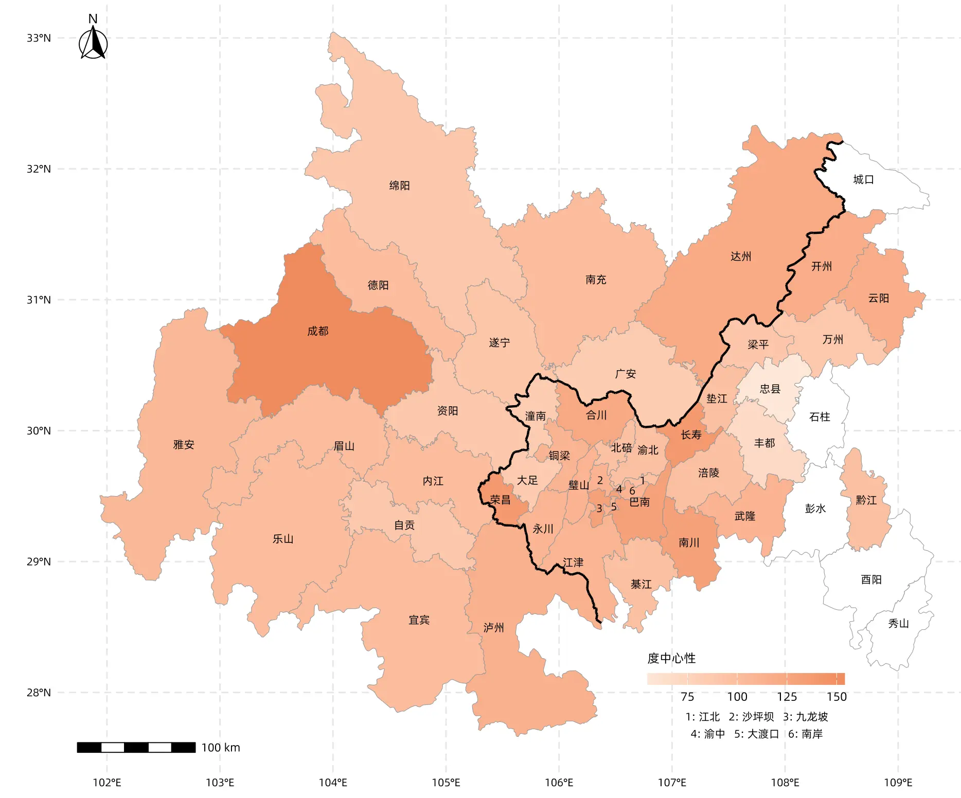

完整代码如下：

# ==============================================================================
# R Script: 成渝双城经济圈社会网络空间分布图 
# ==============================================================================

# ---- Step 1: 加载必要的包 ----
library(sf)
library(ggplot2)
library(dplyr)
library(readxl)
library(ggspatial)
library(grid)
library(showtext)

# ---- Step 2: 字体设置 ----
showtext_auto()

# 定义您的本地字体路径
my_font_path <- "Data/AlibabaPuHuiTi-2-55-Regular.ttf"
my_font_name <- "Alibaba"

# 注册字体
if (file.exists(my_font_path)) {
  font_add(my_font_name, regular = my_font_path)
  base_font_family <- my_font_name
  message(paste("成功加载本地字体:", my_font_path))
} else {
  warning(paste("未找到字体文件:", my_font_path, "，尝试使用系统默认字体。"))
  tryCatch({
    font_add("Arial", "arial.ttf")
    base_font_family <- "Arial"
  }, error = function(e) {
    base_font_family <- "sans"
  })
}


# ---- Step 3: 读取地理数据 ----
tryCatch({
  cities_data <- st_read("China Map/中国_市.geojson", quiet = TRUE)
  districts_data <- st_read("China Map/中国_县.geojson", quiet = TRUE)
  message("GeoJSON 地图文件读取成功。")
}, error = function(e) {
  stop("读取 GeoJSON 失败，请检查 'China Map' 文件夹。错误: ", e$message)
})


# ---- Step 4: 定义目标区域 ----
target_areas_cities_cn <- c("成都市", "绵阳市", "宜宾市", "德阳市", "南充市", "达州市", 
                            "泸州市", "乐山市", "自贡市", "眉山市", "遂宁市", "内江市", 
                            "广安市", "雅安市", "资阳市")

target_areas_districts_cn <- c("渝北区", "渝中区", "九龙坡区", "沙坪坝区", "南岸区", "江津区", 
                               "北碚区", "巴南区", "涪陵区", "璧山区", "万州区", "永川区", 
                               "长寿区", "合川区", "大渡口区", "铜梁区", "大足区", "綦江区", 
                               "荣昌区", "开州区", "潼南区", "梁平区", "南川区", "云阳县", 
                               "忠县", "垫江县", "黔江区", "丰都县", "石柱土家族自治县", 
                               "彭水苗族土家族自治县", "武隆区", "城口县", 
                               "秀山土家族苗族自治县", "酉阳土家族苗族自治县", "江北区")

gb_code_for_jiangbei <- '156500105'


# ---- Step 5: 筛选与清洗数据 ----
sichuan_cities <- cities_data %>% 
  filter(name %in% target_areas_cities_cn) %>%
  mutate(name = trimws(name))

chongqing_districts <- districts_data %>% 
  filter((name %in% target_areas_districts_cn & name != "江北区") | 
           (name == "江北区" & gb == gb_code_for_jiangbei)) %>%
  mutate(name = trimws(name))

sichuan_chongqing <- rbind(sichuan_cities, chongqing_districts) %>%
  distinct(name, .keep_all = TRUE)


# ---- Step 6: 读取 Excel 指标数据 ----
excel_path <- "Output.bk/分类指标社会网络分析结果.xlsx"
node_data_for_plot <- NULL

if (file.exists(excel_path)) {
  tryCatch({
    node_data <- read_excel(excel_path, sheet = "Node_Data")
    if (all(c("Node", "度中心性") %in% names(node_data))) {
      node_data_for_plot <- node_data %>%
        select(Node, `度中心性`) %>%
        rename(name = Node, value_to_plot = `度中心性`) %>%
        mutate(name = trimws(name), value_to_plot = as.numeric(value_to_plot)) %>%
        filter(!is.na(value_to_plot))
      message("Excel 指标数据读取成功。")
    }
  }, error = function(e) { warning("Excel读取出错: ", e$message) })
}


# ---- Step 7: 合并数据 ----
if (!is.null(node_data_for_plot)) {
  sichuan_chongqing <- sichuan_chongqing %>% left_join(node_data_for_plot, by = "name")
} else {
  sichuan_chongqing$value_to_plot <- NA
}


# ---- Step 8: 计算中心点并处理标签 (包含忠县特定修复) ----
sichuan_chongqing_centroids <- suppressWarnings(st_point_on_surface(sichuan_chongqing))

chongqing_core_cn <- c("江北区", "沙坪坝区", "九龙坡区", "渝中区", "大渡口区", "南岸区")
chongqing_core_labels <- c("1", "2", "3", "4", "5", "6")
core_mapping <- setNames(chongqing_core_labels, chongqing_core_cn)

sichuan_chongqing_centroids <- sichuan_chongqing_centroids %>%
  mutate(
    # 1. 核心区转数字
    label = ifelse(name %in% chongqing_core_cn, core_mapping[name], name),
    
    # 2. 通用简化规则 (成都市 -> 成都, 忠县 -> 忠)
    label = ifelse(label %in% chongqing_core_labels, label, {
      temp <- label
      temp <- gsub("土家族|苗族|自治县", "", temp)
      temp <- gsub("[市区县]$", "", temp)
      temp
    }),
    
    # 3. 【特定修复】如果原名是"忠县"，强制改为"忠县" (覆盖掉上面的通用规则)
    label = ifelse(name == "忠县", "忠县", label)
  )

message("标签处理完成 (忠县已单独修正)。")


# ---- Step 9: 计算共享边界 ----
shared_boundary <- NULL
tryCatch({
  sc_proj <- st_transform(st_make_valid(sichuan_cities), 3857)
  cq_proj <- st_transform(st_make_valid(chongqing_districts), 3857)
  
  sc_bound <- st_boundary(st_union(sc_proj))
  cq_bound <- st_boundary(st_union(cq_proj))
  
  shared_proj <- st_intersection(sc_bound, cq_bound)
  
  if (!st_is_empty(shared_proj)) {
    shared_boundary <- st_transform(shared_proj, 4326)
  }
}, error = function(e) { warning("共享边界计算失败: ", e$message) })


# ---- Step 10: 坐标转换 ----
target_plot_crs <- 4326
sichuan_chongqing <- st_transform(sichuan_chongqing, target_plot_crs)
sichuan_chongqing_centroids <- st_transform(sichuan_chongqing_centroids, target_plot_crs)


# ---- Step 11: 绘图 ----
annotation_text <- "1: 江北   2: 沙坪坝   3: 九龙坡\n4: 渝中   5: 大渡口   6: 南岸"
annotation_grob <- textGrob(
  label = annotation_text,
  hjust = 0.5, vjust = 0.5, 
  gp = gpar(fontsize = 8, fontfamily = base_font_family, lineheight = 1.3)
)

map_plot <- ggplot() +
  # 底图
  geom_sf(data = sichuan_chongqing, aes(fill = value_to_plot), 
          color = "gray60", linewidth = 0.2) +
  
  # 共享边界
  { if (!is.null(shared_boundary)) 
    geom_sf(data = shared_boundary, color = "black", linewidth = 0.8) 
  } +
  
  # 标签
  geom_sf_text(data = sichuan_chongqing_centroids, aes(label = label),
               size = 2.8, color = "black", family = base_font_family,
               check_overlap = FALSE) + 
  
  # 指北针
  annotation_north_arrow(location = "tl", which_north = "true",
                         pad_x = unit(0.3, "cm"), pad_y = unit(0.5, "cm"),
                         height = unit(1.2, "cm"), width = unit(1.2, "cm"),
                         style = north_arrow_fancy_orienteering) +
  
  # 比例尺
  annotation_scale(location = "bl", width_hint = 0.25,
                   pad_x = unit(0.5, "cm"), pad_y = unit(0.5, "cm"),
                   text_family = base_font_family) +
  
  # 颜色条
  scale_fill_gradient(name = "度中心性", 
                      low = "#FDE7D7", high = "#F08B5D",
                      na.value = "white",
                      guide = guide_colorbar(direction = "horizontal",
                                             title.position = "top",
                                             barwidth = unit(10, "lines"),
                                             barheight = unit(0.6, "lines"))) +
  
  # 核心区说明
  annotation_custom(
    grob = annotation_grob,
    xmin = 106.5, xmax = 109,
    ymin = 27.5, ymax = 28.0
  ) +
  
  # 主题
  theme_minimal(base_family = base_font_family) +
  theme(
    axis.title = element_blank(),
    axis.text = element_text(color = "black", size = 8, family = base_font_family),
    panel.grid.major = element_line(color = "grey90", linetype = "dashed"),
    legend.position = c(0.75, 0.12), 
    legend.background = element_blank(),
    legend.title = element_text(size = 9, face = "bold", family = base_font_family),
    plot.margin = unit(c(0.5, 0.5, 0.5, 0.5), "cm")
  ) +
  
  # 坐标系
  coord_sf(crs = target_plot_crs, clip = "off")


# ---- Step 12: 输出 ----
print(map_plot)
'''